Evaluation of the Efficiency of Neural Networks and Statistical Models to Determine Daily Traffic Volume of the Suburban Roads of Mazandaran Province
Sepideh Gholampour Shahab Aldini1 * , Shahriar Afandizadeh Zargar2 and Seyed Mohammad Seyed Hoseini3
1
Department of Transportation Engineering,
Science and Research Branch,
Islamic Azad University,
Tehran,
Iran
2
Civil Engineering Department,
Iran University of Science and Technology,
Iran
3
Professor Industrial Engineering Department,
Iran University of Science and Technology,
Iran
http://dx.doi.org/10.12944/CWE.10.Special-Issue1.28
Realizing the traffic volume at the present time is frequently one of the concerns that occupies the planners’ minds in transportation. Knowing the current volume plays an important role in reflecting the performance of transportation system in the future. Traffic studies are based on observations and interpretations of the current circumstances .Since the present observations cannot be represented for the future status, it should be predicted by means of determined conditions. Annual Average Daily Traffic is one the measure to be used for the traffic volume, which has been mentioned in the codes. The fixed or non-fixed automated counters serve to count this volume. In Iran, Road Maintenance & Transportation Organization is responsible to count daily through different ways. In the present study, the data collected from the selected axes of Mazandaran Province was utilized to make a predictive model for traffic volume. It is fitted by data, linear and logarithmic regression models and also neural network model.
Copy the following to cite this article:
Zargar S. A, Aldini S. G. S, Hoseini S. M. S. Evaluation of the Efficiency of Neural Networks and Statistical Models to Determine Daily Traffic Volume of the Suburban Roads of Mazandaran Province. Special Issue of Curr World Environ 2015;10(Special Issue May 2015). DOI:http://dx.doi.org/10.12944/CWE.10.Special-Issue1.28
Copy the following to cite this URL:
Zargar S. A, Aldini S. G. S, Hoseini S. M. S. Evaluation of the Efficiency of Neural Networks and Statistical Models to Determine Daily Traffic Volume of the Suburban Roads of Mazandaran Province. Special Issue of Curr World Environ 2015;10(Special Issue May 2015). Available from: http://www.cwejournal.org?p=668/
Download article (pdf)
Citation Manager
Publish History
Introduction
This Prediction of travelling rate was the primary data enjoying complexity in this present study. It has frequently been discussed on specifying how many travels occur in a particular region and condition whereas has been introduced new methods to predict it. Making model is the most important methods that are utilized by researchers’ model to discover the specific relationships embedded in the data. The directly predictive techniques are those attempt to predict frequency volume as a model; for instance, mathematic model and indirect methods predict the demand for travelling by calling upon 4-level models in the traffic solutions.
The present study included 5 sections: the first section focused on intruding the study. Afterwards, the famous authors’ works and related books were reviewed.
In section three, the researcher talks about the participants and instruments which were used in order to examine the hypotheses. In section four, making linear and logarithmic Regression models and neural network were called upon.
The closure to the study will be done by drawing conclusions.
Review of Related Literature
It has been demanded so much about predicting the annual average daily traffic (AADT) (hence traffic volume is used instead) that is divided into two groups:
The first group is related to a series of researches that estimate the traffic volume at the present time and the second one is related to investigations that attempt to predict traffic volume; for instance, in 1983 Neveu [1] made use of population parameters such as : car ownership, number of households and number of professionals to predict traffic volume.in 1998,Mohammad and et al[2] utilized multiple regression .such as population, type of that route, accessibility to the similar routs and mileage of arterial routs in order to make model in estimating traffic volume.
In 2001, Zaho and Chang [3] generated a model consisting of multiple regressions by means of calculating the number of lines, land use, type of route and socioeconomic conditions. In 2000, Seaver [4] utilized the data collected from 80 regions of Georgia states to estimate the traffic volume of the suburban routes. He employed 42 parameters of Principal Component Analysis to find the effective parameters; in the next step he used regression clustering to identify the similar groups and finally he find a model for each cluster of regression, which enjoys the most efficient traffic volume estimation.
Methodology
The proposed structure for model of estimating volume was demonstrated in the figure 1.As seen in this figure, at first we reviewed the previous studies and extracted the variables relating to traffic prediction and then structure of model by means of linear and logged regression would be used and finally investigated the model.
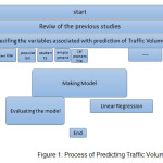 |
Fig. 1: Process of Predicting Traffic Volume Click here to View figure |
The term "regression" was coined by Francis Galton in the nineteenth century to describe a biological phenomenon. The phenomenon was that the heights of descendants of tall ancestors are likely to regress down towards a normal average (a phenomenon also known as regression toward the mean).[5][6] For Galton, regression had only this biological meaning,[7] but his work was later extended by Udny Yule and Karl Pearson to a more general statistical context. [8][9] In the work of Yule and Pearson, the joint distribution of the response and explanatory variables is assumed to be Gaussian. This assumption was diluted by R.A. Fisher in his works of 1922 and 1925. [8] Fisher assumed that the conditional distribution of the response variable is Gaussian, but the joint distribution need not be.[9]
Regression Models are used for the intentions such as describing data, estimation of the parameters and prediction.
Regression models involve the following variables:
- The unknown parameters, denoted as β, which may represent a scalaror a vector.
- The independent variables, X.
- The dependent variable, Y.
In various fields of application, different terminologies are used in place of dependent and independent variables.
A regression model relates Y to a function of X and β.
Y ≈ f (x, β) (1)
To carry out regression analysis, the form of the function f must be specified. Sometimes the form of this function is based on knowledge about the relationship between Y and X that does not rely on the data. If no such knowledge is available, a flexible or convenient form for f is chosen. Many techniques for carrying out regression analysis have been developed. Familiar methods such as simple linear regression. The adjective simple refers to the fact that this regression is one of the simplest in statistics. it is the most practical as like as multiple linear regression. Simple linear regression fits a straight line in such a way that minimalize the errors. The relationship 2 shows a linear function.
y=a ± bx (2)
In this relationship, a and b stand for constant and slope, respectively. In multivariable or combining linear regression can be represented in this general form:
y = β0 + β1x1 + β2x2+…+ βp-1xp- 1+ε (3)
In which x1, x2… xp-1 are independent variables, β0, β1… βp-1 are regression coefficients and ε stands for error.[10]
Linear Regression
Multiple linear regression attempts to model the relationship between two or more explanatory variables and a response variable by fitting a linear equation to observed data. Every value of the independent variable x is associated with a value of the dependent variable y.
y = β0 + β1 x1 + β2 x2 (4)
It is assumed that a logarithmic regression model the normal logarithm Yi follows a normal distribution with the mean µ and variance σ^2. In other words, it is presumed that the given function follows a normal logarithmic distribution.
Lnμ = β0 + β1 Lnxt1 + β2 Lnxt2 + ... βaLn (5)
It is assumed that a logarithmic regression model the normal logarithm Yi follows a normal distribution with the mean µ and variance σ^2. In other words, it is presumed that the given function follows a normal logarithmic distribution.
The coefficients β are linear regressions are calculated through least squares method. It is a classic model taken from a multiple linear relationship between log of dependent variable and predictor or independent variable q.
Neural Network
A neural network is introduced as multiple layers, which is consisted of multiple layers of neurons (including input, hidden or central and output) in a directed graph, with each layer fully connected to the next one.it is trained through a variety of algorithms to carry out various operations. The aim of the present study is applying neural network in non-linear regression, which it is the best alternative for performing such function of MLP networks.
The operations include network training, and then testing the network for training data and also non-training data. Solutions Strategies are used for making decision in line with the existing data in order to introduce the desirable outputs. The neural network does not need to follow specific operational rules whereas requiring a series of data to be trained itself. In order to make neural network models, we have utilized Matlab Software.
Making Model
Prediction of travelling rate is the first-line data used for traffic planning while enjoying a specific complexity. A variety of discussions which have frequently been revolving around specifying how many travels occur in a given region and particular conditions; also, various technique have been proposing on predicting travelling rate. Making model is the utmost techniques that discovers the determined relationships embedded into the present data.
Dependent and Independent Variables in Model
In making model for predicting traffic volume, several variables are called upon. Such variables can be divided into the following classifications:
The economic variables including the average income of households, Car ownership, etc.
The social variables including population, rate of employment, etc.
Traffic variables including the number of lanes, speed, etc.
Environmental variables including land use, access to the available routs
The primary variables in this study include population, employment rate, number of students, fuel consumption, number of households, the number of sickbeds and the average income of the households. As a matter of fact, the data of the studied axes are collected by means of mechanical counting devices, which recorded in Mazandaran Province Road Maintenance & Transportation Organization and statistic yearbook for the studied axes over the past 5 years. Also it should be mentioned that the variables including number of households, average income of the households and the rate of employment have been omitted because of contradictions in their reports; hence, population, rate of employment, number of students and fuel consumption are the variables for the present study.
Correlation coefficient is a mathematical indication to describe the direction and value of a relationship between two variables. To test correlation, different coefficients are used, which simple Pearson correlation is one of them. The Pearson Correlation Test serves to select the most effective variable from other ones that are linearly and strongly correlated. For this reason, the volume of vehicle traffic has been viewed as a dependent variable and the others have been independent variables. We have employed SPSS software to make the linear model and conduct tests for its ability in processing data.
The volume of vehicle traffic is Y, population is X2, sickbeds is X3 and consumption (1000 cubic meters) is X4.
At first we have verified the normality of data after calculating the correlation between dependent variable with other variables by applying Sig coefficient, namely P- value.
In this phase of the study, the significant level for the test is .005 (this value is .005 or .001 in Pearson Test), the parameters being lower than this value can have a correlation with the dependent variable.
According to the significant level seen, correlation between traffic volume and consumption, sickbeds and population is lower than .005, but this is not taken place for employment rate, thus we omit this variable to proceed making model. And finally we have reached the desirable model as following:
V: volume of vehicle traffic
Po: Population
St: Student
Hb: Number of sickbeds
Fu: Consumption
Data Collection
As a matter of fact, the data of the studied axes are collected by means of automated traffic counter, which recorded in Mazandaran Province Road Maintenance & Transportation Organization and statistic yearbook for the studied axes over the past 5 years; it is also available in the site of this organization.
Moreover, by hiring an observer to record traffic in a specified time, we have determined value of traffic volume and then it has been subtracted from the total traffic volume to produce a model based on volume of vehicle traffic from origin to destination.
Several parameters being important in the traffic volume of the axes might not be included wholly due to the limitation in accessing to all of the data. In the present study, the socioeconomic features of origin and destination were not taken into considerations, such as population, number of sickbeds, students and fuel consumption to study on traffic, analyze the trend and predict the future conditions.
Sari to Ghaemshahr axis ,as the second place in Iran’s traffic volume in the suburban, a separated two-lane,22 kilometers, was selected. In fact the course of Sari to Ghaemshahr was just taken into consideration in this study.
Babol to Ghaemshahr axis was a separated two-lane highway to be investigated in this study but we just consider the course of Babol to Ghaemshahr. This axis was 20 kilometers.
Sari to Neka Axis was a separated two-lane highway to be investigated. It was about 20 kilometers. We considered the course of Neka to Sari in this study. And the last axis to be investigated in this study was Babolsar to Babol that was about 20 kilometers and it was a separated two-lane highway.
4-3 Regression Method is used for analyzing the relationships between independent variables to develop a dependent variable. This relationship follows a function. The form and type of the function is determined based on the precision of predictions and we select a function that shows minimum errors would be selected as a target function.
Making a Linear Regression Model
At first making a linear regression model was practiced on the data. The dependent data in
This state is the two-way passing a specific point in a 24-hour period and we demonstrate the results in the following table. This table consists of variables of the model, coefficients-statistics and P-value, which are summary of statistics of the model. Also the confidence level for determining significance of the variables was 95%.Table 1 shows the model fitting results
Table1: The Results fitting Linear Regression
| Model | Calculated coefficients | Sig. | |
| B | |||
| 1 | (Constant) | 10499.308 | .059 |
| Poi | .000 | .143 | |
| Hbi | -26.471 | .097 | |
| Sti | 1.431 | .071 | |
| Fui | 107.405 | .010 | |
| Poj | .001 | .106 | |
| Hbj | 28.460 | .045 | |
| Stj | -1.022 | .033 | |
| Fuj | -53.232 | .055 | |
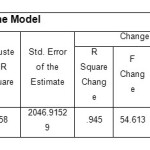 |
Table 2: summary of the Model Click here to View table |
Adjusted R square calculated from the model shows the linear proper relationship between the dependent variable and independent variables; in other words the model (variables with the calculated coefficients) is about 90 %of the dependent coefficient. Plus, it should be noted that the model was verified by the F-statistics. The general form of corresponds to relationship 6.The following points mentioned in the table can be interpreted as:
v = 6255.2 + .001Po - 8.4 Hb + 184.432 Fu + 0.167 St (6)
Table3: linear regression model fitting the results
| Model | Unstandardized Coefficients | T | Sig. | |
| B | ||||
| 2 | (Constant) | 2.648 | 1.236 | .242 |
| LnPoi | .017 | .380 | .711 | |
| LnHbi | .282 | 1.494 | .163 | |
| LnSti | -.067 | -.535 | .603 | |
| LnFui | .574 | 4.220 | .001 | |
| LnPoj | .009 | .220 | .830 | |
| LnHbj | .356 | 2.795 | .017 | |
| LnStj | .178 | .816 | .432 | |
| LnFuj | -.155 | -.820 | .430 | |
The ultimate form would be
V = 47165 + 1242.31 LnPo - 80.4 LnHb + 12582.86 LnFu + 30.246St (7)
Making Neural Network Model
The input consists of population data, number of sickbeds, number of students, number of professionals and fuel consumption. In order to attain a proper architecture, the coded network is run in the central layer with number of the different neurons to reach the best architecture from the minimum errors. The best architecture of network that is used as 5-20-1-1 or 5 inputs,20 neurons in the first central layer and 1 neuron in the second central layer.
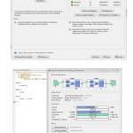 |
Fig. 2: Output Click here to View figure |
In the second state, we selected the cities revolving the axes, which was studied, to investigate the frequency of moves. The above figure shows the setting and the structure of the network, while the number of data was increasing regarding to the number of cities. The architecture of the network was seen as 5-20-1-1 whereas utilizing code writing to execute software. As seen, the software was repeated after 567 times to find the desirable answer that was acceptable regarding to a few number of data
Table4: Summery of the model
| Model | R | R Square | Adjusted R Square | Std. Error of the Estimate | Change Statistics | Durbin-Watson | ||||
| R Square Change | F Change | df1 | df2 | Sig. F Change | ||||||
| 1 | .993a | .957 | .977 | .07600 | .957 | 101.453 | 8 | 11 | .000 | 1.424 |
Table5: the results of making model
| Method | R2 | |
| Frequency of Access | Linear Regression | .905 |
| Logarithmic Regression | .904 | |
| Neural Network | ,949 | |
| Frequency of Movement | Linear Regression | .898 |
| Logarithmic Regression | .922 | |
| Neural Network | ,864 |
Conclusion
In this study. We have suggested an artificial neural network and regression.
Regression has been more practical in most field of study .output of making model and regression are the two advanced regressions such as linear and logarithmic regressions. The two model were selected based on type and number of data. The results of linear model R2 was 0.905 and the logarithmic model was .941 and for the second such value was .898 and .922 ,respectively. as a matter of fact the results were acceptable although the number of data was limited, i.e., the more we had number, the more we enjoy precision. The R2 that was supported by artificial neural network was .949 for the first state and .864 for the second state, and it showed an ability of neural network to support various data.
The results showed that the models enjoyed a high precision to specify traffic access. That is why such routs in Mazandaran Province were used for car traffic within province and also employed as an inter-province car traffic.
The results indicated that artificial intelligence functions can contribute to improve prediction and prediction, but it should be noted that growing in number of population can help researchers to increase the reliability of models. At any rate, it was seen that artificial neural network functioned more efficient than the basic and typical methods.
Reference
- Neveu, A., Quick response procedures to forecast rural traffic, In Transportation Research Record, 944 Washington DC: Transportation Research Board, (1983).
- Mohamad, D., Sinha, K.C., Kuczec, T. and Scholer, C.F., Annual average daily traffic prediction model for county roads,” In Transportation research record, 1617, Washington, DC: Transportation Research Board.(1998).
- Zhao, F. and Chung, S., Contributing factors of annual average daily traffic in a lorida county: Exploration with geographical information system and regression model,” In Transportation research record, 1769, Washington DC: Transportation Research Board, (2001).
- Seaver, W.L., Chatterjee, A. and Seaver, M.L., Estimation of traffic volume on rural local roads,” In Transportation research record, 1719, Washington DC: Transportation Research Board, (2000).
- Castro-Neto, M., Jeong, Y., Jeong, M.K. and Han, L.D., AADT prediction using support vector regression with data-dependent parameters, Department of Civil and Environmental Engineering, University of Tennessee, Knoxville, TN 37996, USA, (2008).
- Witten, I. and Frank, E., Data Mining: Practical Machine Learning Tools and Techniques, university of Waikato, Hamilton, New Zealand, (2010).
- F. Gauss. Theoria combinationis observationum erroribus minimis obnoxiae. (1821/1823)
- Galton F. Presidential address, Section H, Anthropology. (Galton uses the term "regression" in this paper, which discusses the height of humans.), (1885).
- Yule, G. Udny, On the Theory of Correlation". J. Royal Statist. Soc. (Blackwell Publishing) 60 (4): 812–54, (1897).
- Pearson, K. Yule, G.U. Blanchard, N. and Lee, A., The Law of Ancestral Heredity. Biometrika (Biometrika Trust) 2 (2): 211–236, (1903).